The loss functions: rho, psi, weight
An MM-estimator is fully determined by three things: the loss rho(u)
applied to scaled residuals u = r / sigma, its derivative the
influence function psi = rho', and the IRWLS weight
w(u) = psi(u) / u that actually shows up inside the weighted-least-squares
step. They are the same object viewed three ways.
Two properties matter:
rhoshould be bounded so outliers cannot contribute arbitrarily to the objective. This is what gives a high breakdown point.psishould be redescending: zero outside some threshold, so the weightpsi(u) / usmoothly drives extreme residuals to weight zero. That is what gives high Gaussian efficiency at the M-step.
robustbase’s lmrob (and so pylmrob) ships six redescending families:
bisquare, welsh, optimal, hampel, lqq, ggw. huber is
also available for M-only work but is excluded from the S-step because
it is not redescending. The plots below make the shapes concrete.
import numpy as np
import matplotlib.pyplot as plt

from pylmrob import psi as P

plt.rcParams.update({"figure.dpi": 110, "axes.grid": True, "grid.alpha": 0.3})

# Tuning constants, taken directly from robustbase via pylmrob.control.
# M-step tuning targets 95% Gaussian efficiency.
# S-step tuning targets 50% breakdown point.
TUNING_M = {
    "bisquare": (4.685061,),
    "welsh":    (2.11,),
    "optimal":  (1.060158,),
    "hampel":   (1.5 * 0.9016085, 3.5 * 0.9016085, 8.0 * 0.9016085),
    "lqq":      (1.4734061, 0.9826779, 1.5),
    "ggw":      (1.0, 1.5, 0.5, 1.694),
}
TUNING_S = {
    "bisquare": (1.547645,),
    "welsh":    (1.0 / np.sqrt(3.0),),
    "optimal":  (0.4047,),
    "hampel":   (1.5 * 0.2119163, 3.5 * 0.2119163, 8.0 * 0.2119163),
    "lqq":      (0.4015457, 0.2676971, 1.5),
    "ggw":      (1.0, 1.5, 0.5, 0.4375470),
}

FAMILIES = list(TUNING_M)
COLORS = dict(zip(FAMILIES, ["#1f77b4", "#ff7f0e", "#2ca02c",
                             "#d62728", "#9467bd", "#8c564b"]))
u = np.linspace(-6.0, 6.0, 401)
The three views, side by side
def plot_triplet(tuning, title):
    fig, axes = plt.subplots(1, 3, figsize=(13, 3.6), sharex=True)
    for fam in FAMILIES:
        k = tuning[fam]
        axes[0].plot(u, P.rho(u, fam, k), label=fam, color=COLORS[fam])
        axes[1].plot(u, P.psi(u, fam, k), label=fam, color=COLORS[fam])
        axes[2].plot(u, P.wgt(u, fam, k), label=fam, color=COLORS[fam])
    axes[0].set_title("rho(u)  -- loss")
    axes[1].set_title("psi(u)  -- influence")
    axes[2].set_title("w(u) = psi(u)/u  -- IRWLS weight")
    for ax in axes:
        ax.axvline(0, color="black", lw=0.5)
        ax.set_xlabel("u = r / sigma")
    axes[2].legend(loc="upper right", fontsize=8)
    fig.suptitle(title)
    fig.tight_layout()
    plt.show()

plot_triplet(TUNING_M, "M-step tuning (95% Gaussian efficiency)")
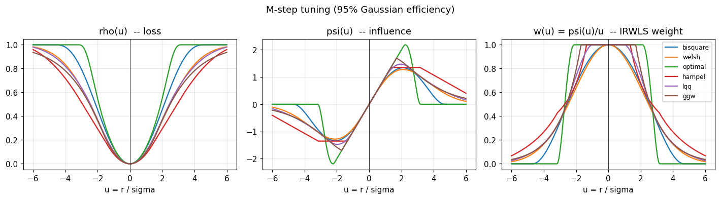
All six losses look similar near zero (so well-behaved points are treated
almost like OLS) and flatten out beyond their respective bend points (so
gross outliers contribute a bounded amount). The psi panel makes the
“redescending” property concrete: every curve returns to zero outside its
threshold, which forces the weight in the right panel to fall to zero as
well. hampel is the only piecewise-linear family in the set, which is
why its psi has visible corners.
Now the same families at the S-step tuning. The shapes are identical;
the curves are just rescaled so the bend points sit much closer to the
origin. That smaller scale is what makes the S-step’s objective concentrate
on the bulk of the data and ignore everything past ~2 sigma.
plot_triplet(TUNING_S, "S-step tuning (50% breakdown)")
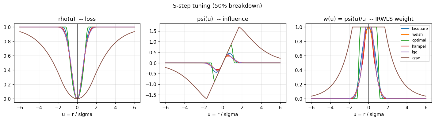
Why MM uses two tunings
The same family is used at both the S-step and the M-step, but with different tuning constants. The S-step needs the narrowest possible bend to push the breakdown point up to 50%, and pays for that with low Gaussian efficiency (around 28%). The M-step starts from the S-step’s solution and widens the bend until it reaches 95% efficiency on clean data. Plotting bisquare at both tunings makes the trade-off visible.
fig, axes = plt.subplots(1, 3, figsize=(13, 3.6), sharex=True)
for label, k, color, ls in [
    ("S-step (k=1.548, 50% bp, ~28% eff)", 1.547645, "#d62728", "-"),
    ("M-step (k=4.685, 95% eff)", 4.685061, "#1f77b4", "--"),
]:
    axes[0].plot(u, P.rho(u, "bisquare", (k,)), label=label, color=color, ls=ls)
    axes[1].plot(u, P.psi(u, "bisquare", (k,)), label=label, color=color, ls=ls)
    axes[2].plot(u, P.wgt(u, "bisquare", (k,)), label=label, color=color, ls=ls)
axes[0].set_title("rho(u)")
axes[1].set_title("psi(u)")
axes[2].set_title("w(u) = psi(u)/u")
for ax in axes:
    ax.axvline(0, color="black", lw=0.5)
    ax.set_xlabel("u = r / sigma")
axes[0].legend(loc="lower right", fontsize=8)
fig.suptitle("bisquare: S-step vs M-step tuning")
fig.tight_layout()
plt.show()
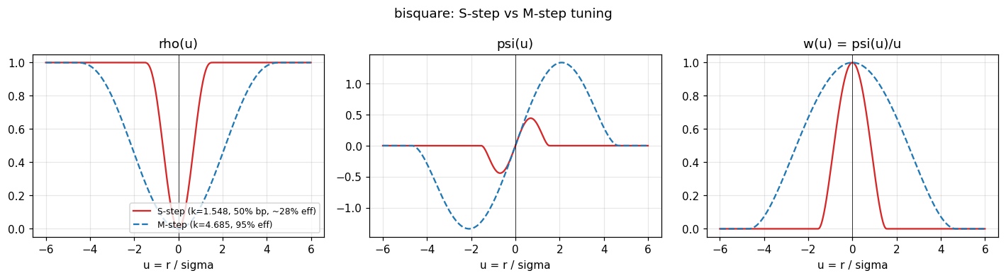
The wide M-step weight gives near-OLS behavior on observations within
roughly 4.7 sigma. The narrow S-step weight is what does the heavy
lifting against outliers: anything past ~1.5 sigma is fully discarded
for the purpose of selecting the scale.
Where huber sits
huber is the historical M-estimator and is not redescending: the
loss grows linearly past its threshold instead of flattening, so the
influence function plateaus at a non-zero value. That is why huber is
allowed for the M-step but not for the S-step or the M-scale equation:
the chi function used by those steps must be bounded.
fig, axes = plt.subplots(1, 3, figsize=(13, 3.6), sharex=True)
k_huber = (1.345,)
k_bisq  = (4.685061,)
axes[0].plot(u, P.rho(u, "huber",    k_huber), label="huber (M-only)", color="#7f7f7f")
axes[0].plot(u, P.rho(u, "bisquare", k_bisq ), label="bisquare",       color="#1f77b4")
axes[1].plot(u, P.psi(u, "huber",    k_huber), label="huber",          color="#7f7f7f")
axes[1].plot(u, P.psi(u, "bisquare", k_bisq ), label="bisquare",       color="#1f77b4")
axes[2].plot(u, P.wgt(u, "huber",    k_huber), label="huber",          color="#7f7f7f")
axes[2].plot(u, P.wgt(u, "bisquare", k_bisq ), label="bisquare",       color="#1f77b4")
axes[0].set_title("rho(u)")
axes[1].set_title("psi(u)")
axes[2].set_title("w(u)")
for ax in axes:
    ax.axvline(0, color="black", lw=0.5)
    ax.set_xlabel("u = r / sigma")
axes[0].legend(loc="lower right", fontsize=8)
fig.suptitle("huber (non-redescending) vs bisquare (redescending)")
fig.tight_layout()
plt.show()

Huber’s psi saturates at +/- k instead of returning to zero. The
weight stays at 1/|u| for large |u|, so an outlier always retains
some influence: it is downweighted, not discarded. That bounded influence
is enough for an M-fit on clean designs but not enough to defend against
high-leverage contamination, which is the gap MM closes by adding the
S-step on top.
Next
Pick the family you want by passing psi= to Control:
from pylmrob import Control, lmrob
fit = lmrob("y ~ x", df, control=Control(psi="lqq"), seed=42)
The default is bisquare; setting="KS2014" switches to lqq. See the
FAQ for guidance on when to pick a non-default family and
notebook 04 for how these losses feed into the S +
MM pipeline.