Why robust at all?
Two kinds of outliers can wreck an OLS fit:
Vertical outliers — a few rows have wildly wrong
yvalues. Thex’s are fine.Horizontal (high-leverage) outliers — a few rows sit far from the bulk of the
xdistribution AND have wrongy. These are the dangerous ones: theirx-position gives them disproportionate influence on the OLS solution.
This notebook compares four estimators on each scenario:
OLS (
statsmodels.OLS): the baseline.MM-estimator (
pylmrob.lmrob): bounded loss + S-init.Huber-M (
statsmodels.RLMwithHuberT): a plain M-estimator, bounded loss but no high-breakdown init.Theil-Sen (
sklearn.linear_model.TheilSenRegressor): median-of-pairwise-slopes; high breakdown by construction.
The point is to see the failure modes, not just hear about them.
import numpy as np
import matplotlib.pyplot as plt
import pandas as pd

from pylmrob import lmrob, Control
import statsmodels.api as sm
from statsmodels.robust.robust_linear_model import RLM
from sklearn.linear_model import TheilSenRegressor

rng = np.random.default_rng(0)

# Shared style
plt.rcParams.update({"figure.dpi": 110, "axes.grid": True, "grid.alpha": 0.3})

METHOD_COLORS = {
    "OLS": "#d62728",
    "MM (pylmrob)": "#1f77b4",
    "Huber-M": "#ff7f0e",
    "Theil-Sen": "#2ca02c",
}
Helper
A single function that fits all four methods and returns
(intercept, slope) per method on a 1-D regression problem.
def fit_all(x, y):
    """Fit OLS / MM / Huber-M / Theil-Sen on (x, y); return dict of (b0, b1)."""
    X = sm.add_constant(x)
    out = {}

    # OLS
    res = sm.OLS(y, X).fit()
    out["OLS"] = (res.params[0], res.params[1])

    # MM-estimator (pylmrob default = bisquare, S init, 50% breakdown)
    df = pd.DataFrame({"x": x, "y": y})
    fit = lmrob("y ~ x", df, control=Control(), seed=42)
    out["MM (pylmrob)"] = (fit.coef_[0], fit.coef_[1])

    # Huber-M (statsmodels)
    rlm = RLM(y, X, M=sm.robust.norms.HuberT()).fit()
    out["Huber-M"] = (rlm.params[0], rlm.params[1])

    # Theil-Sen (sklearn)
    ts = TheilSenRegressor(random_state=0).fit(x.reshape(-1, 1), y)
    out["Theil-Sen"] = (ts.intercept_, ts.coef_[0])

    return out


def plot_panel(ax, x, y, fits, title, true_intercept, true_slope):
    """Scatter + four regression lines."""
    ax.scatter(x, y, s=18, alpha=0.6, color="black", label="data")
    xs = np.linspace(x.min(), x.max(), 100)

    # True line (gray dashed)
    ax.plot(xs, true_intercept + true_slope * xs, "--",
            color="gray", lw=1, label="true")

    for method, (b0, b1) in fits.items():
        ax.plot(xs, b0 + b1 * xs, color=METHOD_COLORS[method],
                lw=2, label=method)
    ax.set_title(title)
    ax.set_xlabel("x")
    ax.set_ylabel("y")
    ax.legend(loc="upper left", fontsize=8)
Scenario 1: vertical outliers
We generate a clean linear relationship y = 2 + 1.5x + N(0, 0.5)
on n=100, then corrupt the last 10 responses by replacing them
with values around -20. The x’s are untouched.
n = 100
x = np.linspace(0, 10, n)
y_clean = 2.0 + 1.5 * x + 0.5 * rng.standard_normal(n)

y_vert = y_clean.copy()
y_vert[-10:] = -20.0 + 3.0 * rng.standard_normal(10)

fits_vert = fit_all(x, y_vert)
fits_vert
{'OLS': (np.float64(8.194162039230589), np.float64(-0.46797572863610026)),
 'MM (pylmrob)': (np.float64(1.9610290566646338),
  np.float64(1.5215127971625495)),
 'Huber-M': (np.float64(2.2064921423127544), np.float64(1.4421831475034006)),
 'Theil-Sen': (np.float64(2.1749956878970065), np.float64(1.4555390162287618))}
fig, ax = plt.subplots(figsize=(7, 5))
plot_panel(ax, x, y_vert, fits_vert,
           "Vertical outliers (y-only)",
           true_intercept=2.0, true_slope=1.5)
fig.tight_layout()
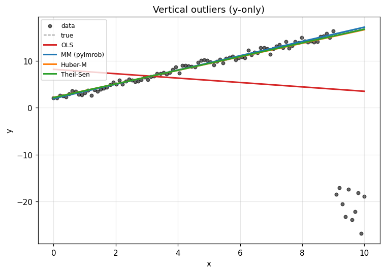
Reading the picture. OLS bends toward the contaminated cluster in the lower right; its slope is roughly flat. The three robust methods recover the underlying line.
Even Huber-M does fine here. The contamination is in y only, so
the leverage structure of the design is clean; downweighting by
residual size is enough.
Scenario 2: horizontal (high-leverage) outliers
Now the harder case. We generate the same clean relationship, but
this time the contamination is in x and y together: a cluster
of 10 points around (x=15, y=0) that sits far to the right of
the main data.
This is the Hawkins-Bradu-Kass structure: the contamination forms its own pseudo-trend that an OLS-style optimizer wants to fit.
x_main = np.linspace(0, 10, 90)
y_main = 2.0 + 1.5 * x_main + 0.5 * rng.standard_normal(90)

# High-leverage cluster: x ≈ 15, y ≈ 0. Far in design space and far below the line.
x_contam = 15.0 + 0.5 * rng.standard_normal(10)
y_contam = 0.0 + 0.5 * rng.standard_normal(10)

x_horiz = np.concatenate([x_main, x_contam])
y_horiz = np.concatenate([y_main, y_contam])

fits_horiz = fit_all(x_horiz, y_horiz)
fits_horiz
{'OLS': (np.float64(7.413812472057469), np.float64(0.19076645686148413)),
 'MM (pylmrob)': (np.float64(2.075331616433327),
  np.float64(1.4839952964380316)),
 'Huber-M': (np.float64(2.5869305558988844), np.float64(1.355800758952904)),
 'Theil-Sen': (np.float64(2.3858231241411176), np.float64(1.4186307641395386))}
fig, ax = plt.subplots(figsize=(7, 5))
plot_panel(ax, x_horiz, y_horiz, fits_horiz,
           "Horizontal (high-leverage) outliers",
           true_intercept=2.0, true_slope=1.5)
fig.tight_layout()
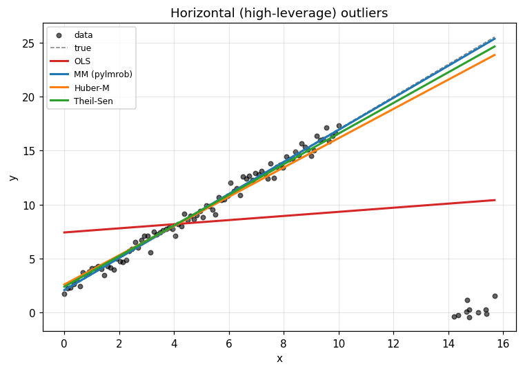
Reading the picture. OLS chases the contamination cluster, so
the slope drops from 1.5 to nearly zero. Huber-M follows OLS:
plain M-estimators downweight by residual size, and a high-leverage
point with a small residual (because the line bends toward it)
keeps a normal weight. The fit gets pulled.
MM recovers the true slope. Its high-breakdown S-init lands in a basin that ignores the contamination cluster, then the MM step refines from there with the high-efficiency tuning.
Theil-Sen also recovers — at the cost of slower fits on larger
problems (O(n²) pairs by default).
This is the practical case for preferring MM over plain M-estimators on real data: in clean designs Huber-M is fine, but the moment a single point lies far in design space, MM’s S-init protects you and Huber-M can’t.
The HBK case study
To close, here is the canonical worst case: the Hawkins-Bradu-Kass dataset (75 obs, 3 predictors, 14 simultaneously high-leverage Y-outliers).
hbk = pd.read_csv("../../tests/data/hbk.csv")
fit = lmrob("Y ~ X1 + X2 + X3", hbk, control=Control(nResample=1000), seed=42)
print("MM coefficients:", dict(zip(fit.term_names_, fit.coef_.round(3))))
print("rows with weight < 0.1:", np.where(fit.rweights_ < 0.1)[0].tolist())
MM coefficients: {'Intercept': np.float64(-0.19), 'X1': np.float64(0.085), 'X2': np.float64(0.041), 'X3': np.float64(-0.054)}
rows with weight < 0.1: [0, 1, 2, 3, 4, 5, 6, 7, 8, 9]
The first 10-14 rows are the contamination block. fit.rweights_
flags them automatically; fit.diagnostics().masked_outliers (the
diagnostic added in v0.5.19) flags the high-leverage subset of those.
diag = fit.diagnostics()
print("masked_outliers (high-leverage AND downweighted):",
      np.where(diag.masked_outliers)[0].tolist())
masked_outliers (high-leverage AND downweighted): [0, 1, 2, 3, 4, 5, 6, 7, 8, 9]
For the diagnostic story on hbk see examples/stackloss_tour
for a richer worked example with the same diagnostics API.
Next
02_efficiency: what does robustness cost on clean data?03_breakdown: how much contamination can each method tolerate?04_s_estimator: why the S-init matters inside MM.