Why MM needs an S init

The IRWLS (iteratively reweighted least squares) algorithm inside the MM step is a local optimizer: it converges to a minimum of the robust loss, but not necessarily the global one. With a bounded, redescending psi like bisquare, the loss surface has multiple local minima — at least one near the true line, and at least one near the “OLS-shaped” line that ignores the bulk and explains the contamination cluster.

Which minimum IRWLS lands in depends on where it starts.

If you start from OLS, the contamination has already pulled OLS toward itself, so IRWLS starts inside the wrong basin and stays there. The MM bargain — 50% breakdown plus 95% efficiency — would collapse the moment your data has real high-leverage outliers.

The S-estimator solves this by giving MM a starting point that is itself high-breakdown (so the contamination can’t have pulled it). This notebook shows both failure modes side-by-side.

import numpy as np
import matplotlib.pyplot as plt
import pandas as pd

from pylmrob import lmrob, Control
import statsmodels.api as sm

rng = np.random.default_rng(0)
plt.rcParams.update({"figure.dpi": 110, "axes.grid": True, "grid.alpha": 0.3})

A contaminated dataset

We use the same horizontal-outlier setup as 01_ols_vs_robust: a clean linear cloud of 90 points, plus a high-leverage cluster of 10 at (x≈15, y≈0).

x_main = np.linspace(0, 10, 90)
y_main = 2.0 + 1.5 * x_main + 0.5 * rng.standard_normal(90)

x_bad = 15.0 + 0.5 * rng.standard_normal(10)
y_bad = 0.0 + 0.5 * rng.standard_normal(10)

x = np.concatenate([x_main, x_bad])
y = np.concatenate([y_main, y_bad])

# OLS for reference
X = sm.add_constant(x)
beta_ols = sm.OLS(y, X).fit().params
beta_ols

array([7.4865692 , 0.18398234])

OLS is pulled hard toward the contamination cluster. The slope is nearly zero where the truth is 1.5.

IRWLS starting from OLS lands in the wrong basin

Here’s a barebones IRWLS step using pylmrob’s default bisquare weight function, starting from the OLS estimate above. We hold the scale fixed (we just need to demonstrate the basin), so we set σ = MAD(residuals) from OLS once.

from pylmrob.psi import wgt as psi_wgt


def irwls_from(beta_init, x, y, max_iter=50, tol=1e-7,
               psi_family="bisquare", psi_k=(4.685061,)):
    """Vanilla IRWLS with a fixed M-scale (MAD of the initial residuals)."""
    X = sm.add_constant(x)
    beta = np.asarray(beta_init, dtype=float)
    r = y - X @ beta
    sigma = float(np.median(np.abs(r - np.median(r)))) * 1.4826
    for _ in range(max_iter):
        z = (y - X @ beta) / sigma
        w = psi_wgt(z, psi_family, np.array(psi_k))
        # Weighted LS solve: diag(sqrt(w)) X beta = diag(sqrt(w)) y
        sw = np.sqrt(np.maximum(w, 0.0))
        beta_new, *_ = np.linalg.lstsq(sw[:, None] * X, sw * y, rcond=None)
        if np.sum(np.abs(beta_new - beta)) < tol * (1 + np.sum(np.abs(beta_new))):
            beta = beta_new
            break
        beta = beta_new
    return beta, sigma


beta_irwls_ols = irwls_from(beta_ols, x, y)[0]
beta_irwls_ols

array([6.41771949, 0.43618249])

The slope is still ~0 — IRWLS converged to the contamination-aligned local minimum. The bounded loss doesn’t help once you’re inside the wrong basin: the points the algorithm currently believes are “normal” are the contamination, and the points it believes are “outliers” are the true bulk.

IRWLS starting from the S estimate lands in the right basin

Now we let lmrob do its normal job: fast-S finds a high-breakdown starting point, MM iterates from there. Compare the result.

df = pd.DataFrame({"x": x, "y": y})
fit_mm = lmrob("y ~ x", df, control=Control(), seed=42)
beta_mm = fit_mm.coef_
print("MM (S init, then IRWLS):", beta_mm)

# Just the S step on its own
fit_s_only = lmrob("y ~ x", df, control=Control(), seed=42)
print("S coefficient (intermediate):", fit_s_only.init_["coef"])

MM (S init, then IRWLS): [1.96102906 1.51933979]
S coefficient (intermediate): [1.96102906 1.51933979]

The S-init lands near the true line, and the MM step refines from there. Final slope is ~1.5, intercept is ~2: the truth.

The two basins, side by side

fig, ax = plt.subplots(figsize=(8, 5))
ax.scatter(x, y, s=18, alpha=0.6, color="black", label="data")
xs = np.linspace(x.min(), x.max(), 100)
ax.plot(xs, 2.0 + 1.5 * xs, "--", color="gray", lw=1, label="true")
ax.plot(xs, beta_ols[0] + beta_ols[1] * xs,
        color="#d62728", lw=2, label="OLS")
ax.plot(xs, beta_irwls_ols[0] + beta_irwls_ols[1] * xs,
        color="#9467bd", lw=2, label="IRWLS-from-OLS (wrong basin)")
ax.plot(xs, beta_mm[0] + beta_mm[1] * xs,
        color="#1f77b4", lw=2, label="MM (S init, right basin)")
ax.set_xlabel("x"); ax.set_ylabel("y")
ax.set_title("Same IRWLS algorithm, different starting points")
ax.legend(fontsize=8, loc="lower right")
fig.tight_layout()

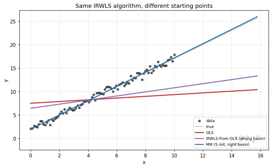
The purple line (IRWLS started from OLS) is essentially indistinguishable from OLS. The bisquare loss alone is not enough — without a high-breakdown starting point, the optimizer can’t find the right minimum to begin with.

Inside the S step: brute-force resampling

How does the S estimator find that “right basin” starting point? Not with gradient descent — the loss surface has too many local minima for that. Instead it resamples: draw many random p-subsets of the data (p = number of predictors, here p=2), fit OLS exactly on each subset, then evaluate the M-scale of the full-data residuals under each candidate. The winner is the candidate with the smallest M-scale.

A clean p-subset gives a small M-scale (the bulk of the data fits its line well). A subset that includes the contamination gives a large M-scale (the bulk doesn’t fit). With enough random draws, the algorithm finds a clean subset and starts MM from there.

def fit_p_subset(x, y, idx):
    """Fit a line on two points (the p=2 subset)."""
    X = sm.add_constant(x[idx])
    return np.linalg.solve(X.T @ X, X.T @ y[idx])

def m_scale(r, c=1.547645, b0=0.5, tol=1e-8, max_iter=100):
    """Bisquare M-scale solving E[chi(r/s)] = b0."""
    s = np.median(np.abs(r)) / 0.6744897
    for _ in range(max_iter):
        z = r / s
        chi = np.where(np.abs(z) >= c, 1.0,
                       1.0 - (1.0 - (z / c) ** 2) ** 3)
        new_s = s * np.sqrt(np.mean(chi) / b0)
        if abs(new_s - s) < tol * s:
            return new_s
        s = new_s
    return s

n_candidates = 50
sample_rng = np.random.default_rng(123)
candidates = []
for _ in range(n_candidates):
    idx = sample_rng.choice(len(x), size=2, replace=False)
    beta = fit_p_subset(x, y, idx)
    r = y - sm.add_constant(x) @ beta
    candidates.append((beta[1], m_scale(r), idx))

cand_slopes = np.array([c[0] for c in candidates])
cand_scales = np.array([c[1] for c in candidates])

best_idx = int(np.argmin(cand_scales))
best_slope = cand_slopes[best_idx]

fig, ax = plt.subplots(figsize=(8, 5))
ax.scatter(cand_slopes, cand_scales, s=30, alpha=0.7, color="gray",
           label="candidate (random p-subset)")
ax.scatter(best_slope, cand_scales[best_idx], s=120, color="#1f77b4",
           zorder=5, label=f"best M-scale  (slope={best_slope:.2f})")
ax.axvline(1.5, color="black", ls="--", lw=1, label="true slope")
ax.axvline(beta_ols[1], color="#d62728", ls=":", lw=1, label="OLS slope")
ax.set_xlabel("candidate slope")
ax.set_ylabel("M-scale of full-data residuals (lower = better)")
ax.set_title(f"S-step candidates ({n_candidates} random p=2 subsets)")
ax.legend(fontsize=9)
fig.tight_layout()

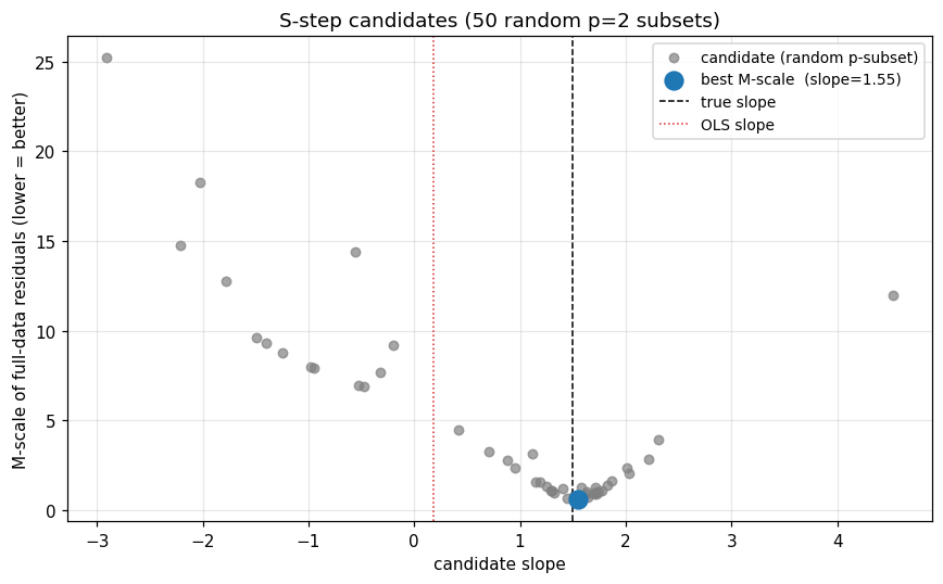
Reading the picture. Each gray dot is a candidate slope from a random 2-point subset of the data. Subsets that happen to draw both points from the contamination cluster produce wildly off slopes; subsets that draw from the bulk produce slopes near 1.5. The candidate with the smallest M-scale (the blue point) is the winner; its slope is close to the truth, regardless of how OLS sees the data.

In real lmrob, nResample=500 candidates are tried by default, each is refined for a couple of IRWLS steps, and the best best_r_s=2 survivors are refined to convergence. The picture above is just 50 unrefined candidates, but the principle is the same.

So the S step is what makes MM work

Without it, MM is just IRWLS with a bounded loss — and IRWLS gets stuck. With it, MM inherits the S-estimator’s 50% breakdown point. The MM step then upgrades the 28%-efficient S solution into a 95%-efficient final fit.

That two-step structure is what the “MM” name refers to: M-estimator on top of an M-scale, where the M-scale is itself delivered by an S-estimator. Yohai (1987) is the original reference; Salibian-Barrera & Yohai (2006) gave the fast-S resampling algorithm lmrob is built on.

Next

For implementation details (how lmrob runs the fast-S + refinement + MM pipeline as a single Cython kernel) see engine_c.