Breakdown point in pictures

The breakdown point of an estimator is the largest fraction of the data you can replace with arbitrary outliers before the estimate becomes useless. It’s a theoretical guarantee, but it has a very concrete operational meaning: sweep contamination from zero to something high, fit your method at each level, and watch where the estimate stops tracking the true value.

Theoretical breakdown points:

Method	Breakdown	Why
OLS	0%	A single huge outlier can move the fit arbitrarily far.
Huber-M	0% in x, ~1/n in y	Bounded loss helps on small-amount Y-only contamination, but no protection against high-leverage points.
Theil-Sen	~29%	Median-of-slopes; breaks once contamination reaches the median.
MM (bisquare default)	50%	The S-init step’s design is half the data; you’d need to corrupt more than half before MM falls.

We’ll measure these by sweeping the contamination fraction.

import numpy as np
import matplotlib.pyplot as plt
import pandas as pd

from pylmrob import lmrob, Control
import statsmodels.api as sm
from statsmodels.robust.robust_linear_model import RLM
from sklearn.linear_model import TheilSenRegressor

rng = np.random.default_rng(0)
plt.rcParams.update({"figure.dpi": 110, "axes.grid": True, "grid.alpha": 0.3})

METHODS = ["OLS", "MM (pylmrob)", "Huber-M", "Theil-Sen"]
COLORS = {
    "OLS": "#d62728",
    "MM (pylmrob)": "#1f77b4",
    "Huber-M": "#ff7f0e",
    "Theil-Sen": "#2ca02c",
}

Setup

For each contamination fraction eps in {0.00, 0.05, 0.10, ..., 0.50}, generate a clean dataset of n=200 then replace floor(eps * n) of the y values with large outliers (y = 50 + N(0, 1)). Fit each method, record the slope. Repeat 25 times per eps and report the median + IQR.

def fit_slope(x, y, method):
    X = sm.add_constant(x)
    if method == "OLS":
        return sm.OLS(y, X).fit().params[1]
    if method == "MM (pylmrob)":
        df = pd.DataFrame({"x": x, "y": y})
        return lmrob("y ~ x", df, control=Control(), seed=42).coef_[1]
    if method == "Huber-M":
        return RLM(y, X, M=sm.robust.norms.HuberT()).fit().params[1]
    if method == "Theil-Sen":
        return TheilSenRegressor(random_state=0).fit(
            x.reshape(-1, 1), y).coef_[0]
    raise ValueError(method)


def contaminate_y(rng, x, true_intercept, true_slope, eps):
    """Generate (x, y) with fraction ``eps`` of y values replaced by outliers."""
    n = len(x)
    y = true_intercept + true_slope * x + 0.5 * rng.standard_normal(n)
    n_bad = int(np.floor(eps * n))
    if n_bad > 0:
        idx = rng.choice(n, size=n_bad, replace=False)
        y[idx] = 50.0 + rng.standard_normal(n_bad)
    return y


def sweep(eps_grid, n_rep=25, n=200, true_intercept=2.0, true_slope=1.5):
    """Return slope estimates as a (len(eps_grid), n_rep, len(METHODS)) array."""
    sim_rng = np.random.default_rng(42)
    x = np.linspace(0, 10, n)
    out = np.empty((len(eps_grid), n_rep, len(METHODS)))
    for i, eps in enumerate(eps_grid):
        for r in range(n_rep):
            y = contaminate_y(sim_rng, x, true_intercept, true_slope, eps)
            for j, m in enumerate(METHODS):
                out[i, r, j] = fit_slope(x, y, m)
    return out


eps_grid = np.linspace(0.0, 0.5, 11)
slopes = sweep(eps_grid)
slopes.shape  # (11, 25, 4)

(11, 25, 4)

Result

median = np.median(slopes, axis=1)            # (11, 4)
q25 = np.quantile(slopes, 0.25, axis=1)       # (11, 4)
q75 = np.quantile(slopes, 0.75, axis=1)       # (11, 4)

fig, ax = plt.subplots(figsize=(8, 5))
for j, m in enumerate(METHODS):
    ax.plot(eps_grid, median[:, j], lw=2, color=COLORS[m], label=m)
    ax.fill_between(eps_grid, q25[:, j], q75[:, j],
                    color=COLORS[m], alpha=0.18)

ax.axhline(1.5, color="gray", ls="--", lw=1, label="true slope")
ax.set_xlabel("contamination fraction ε")
ax.set_ylabel("estimated slope (median ± IQR across 25 reps)")
ax.set_title("Slope estimate vs contamination level")
ax.legend(fontsize=9, loc="lower left")
fig.tight_layout()

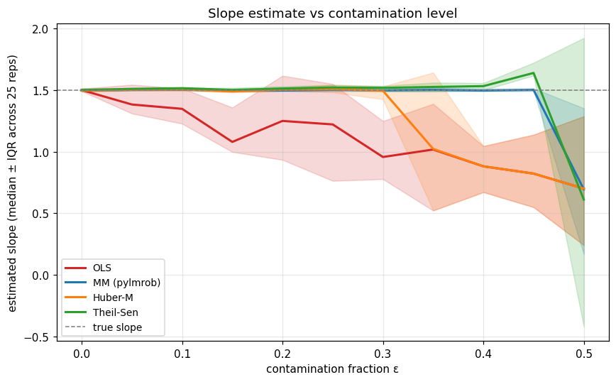
Reading the picture.

• OLS drops the slope linearly. Even at ε=0.05 it’s already off. It has no notion of “outlier”.

• Huber-M holds the slope close to 1.5 for a while — Huber’s bounded loss can absorb a few bad Y values — then drops as the contamination grows past ~25%. Its breakdown point is technically zero (a single bad point at high leverage can ruin it), but in this Y-only contamination scenario the operative bound is a fraction.

• Theil-Sen holds until ε ≈ 0.29 (its theoretical breakdown), then collapses sharply.

• MM stays close to the truth across the entire range. At ε very close to 0.5 it starts to wobble — the S-step’s half-the-data resampling has trouble finding clean half-subsamples — but it remains by far the best of the four.

The “cliff” at the breakdown point isn’t a soft boundary. Once the contamination passes the limit, the estimator’s design assumptions fail and the output is meaningless.

What ε=0.5 means in practice

A 50% breakdown point sounds like a lot of headroom. In real datasets it’s quite ordinary to have 1-5% contamination from data entry errors, sensor glitches, or fat-fingered inputs. The reason to use MM at 50% rather than M at, say, 20% is the distribution in leverage of those errors:

• Y-only contamination (a sensor returns 999 for a missing read, or a typo): Huber-M survives up to maybe 25%.

• Contamination that also moves x (the same sensor returns (999, 999)): Huber-M’s breakdown drops to essentially zero. MM still survives because its S-init protects against leverage.

MM’s 50% breakdown is the worst-case safety net, not a typical operating point.

Next

• 04_s_estimator: why the S step is what makes MM achieve 50% breakdown — and what goes wrong if you skip it.